Update: Megaconstellations in 2023


A year since finishing up my residency I am posting a couple of updates about satellite stats in 2023.

Jonathan McDowell’s Space Activities in 2023
Jan 5, 2024. https://www.planet4589.org/space/

Increasing launches:

    • In 2023 there were 223 orbital launch attempts, and of those 212 reached orbit. This is up from 186 in 2022; 146 in 2021; 114 in 2020; 102 in 2019.

Prominently commercial:

    • Of the 2023 launch attempts, 134 were from commercial companies and for commercial customers, and 78 were from government. The other 11 were contracted by governments and launched by commercial companies.

Leading countries:

    • Deployment of satellites is currently led by USA, China, Russia and Europe, with Japan and India following.

Mostly Comms:

    • Of the satellites launched in 2023 with a mass above 100kg, most are US communication satellites making up mega constellations: 2181 comms satellites (above 100kg) were launched, compared to 67 for Imaging (including weather satellites.)


‘A dynamic shell of conductive material’

‘Potential Perturbation of the Ionosphere by Megaconstellations and Corresponding Artificial Re-entry Plasma Dust’ by S. Solter-Hunt
arXiv, December 6, 2023. http://arxiv.org/abs/2312.09329.

S. Solter-Hunt’s paper describes the alarming potential impact of particles left by satellites in the magnetosphere as they break up on re-entry.

It describes how artificial material left by satellites far outweighs natural quantities of particles in the Earth’s magnetosphere, and the conductive qualities of these satellite materials has the potential to alter the make-up of the magnetosphere which could consequently impact the Earth’s atmosphere.

It states that: “in the 2020s and 2030s, satellites will become so numerous that they will form their own dynamic shell of conductive material.” (Solter-Hunt, 2023, p. 1)

Additionally, Solter-Hunt describes that this is happening at a rate faster than the time it would take to simulate 500,000 satellites in a magnetosphere model.

Therefore: “A simulation of the magnetosphere and the megaconstellations is not currently feasible, and the planetaryscale experiment is underway without a direct ability to diagnose the satellite-magnetosphere relationship because the satellites themselves detect the changes in the magnetic field.” (Solter-Hunt, 2023, p. 1)

The paper concludes: “The space industry on Earth is taking vast amounts of conductive materials naturally found on the surface and in the crust and injecting them into the ionosphere and beyond, causing a new stratification of planetary material.” (Solter-Hunt, 2023, p. 4)

🤯

Update: Bike-tenna

In November, I learnt via Open-Weather that one particular satellite, NOAA15, has a damaged sensor causing degraded data that alters the image composition. I wanted to capture this glitch direct from the satellite, so I went to a bit more effort to avoid the noise I was getting using the antenna on my balcony.

Thanks to an engineer friend, I got hold of a V-dipole antenna which I could attach to my bike and take to a nearby open field (previously, and fittingly, the ‘Starlight’ Drive-in cinema) to escape the household and neighbourhood radio interference.

The images received from NOAA15 have fascinating compositions and image qualities that expands to convey interactions between socio-technical actors on a planetary scale: a faulty US government satellite in dialogue with the social structures that allow me access to a laptop, software, antenna, knowledge, and an open field.

An important reference for this work is Open-weather, led by artist duo Sophie Dyer and Sasha Engelmann, whose ‘Nowcast’ project creates a composite set of NOAA images received from participants around the world. In their paper, ‘Open-weather: Speculative-feminist propositions for planetary images in an era of climate crisis‘ (2022) Dyer and Engelmann describe how empowering people to independently conjure a satellite perspective bypasses the weather channels we normally consult to gauge the atmosphere and creates a ‘counter-image’ that shifts satellite imagery from a scientific to social domain.

Update: Signal to Noise

In 2023 I presented ‘Signal to Noise’ at Canberra Contemporary Artspace (CCAS), combining previous works with a series informed by my ANAT Synapse research.

Signal to Noise, 2023. Installation view, Canberra Contemporary Art Space, 2023. Photograph: Brenton McGeachie.

The major new work, ‘Sent to the sky, received from the stars’ is a military surplus parachute printed on using the cyanotype process. It creates a composite of perspectives of looking up and down to and from satellites, in a form that alludes to position of orbital space as instrumental in both weather, and war.

Sent to the sky, received from the stars, 2023, cyanotype on parachute, nylon, silk, dimensions variable. Installation view, Canberra Contemporary Art Space, 2023. Photograph: Brenton McGeachie.

The printed imagery creates a composite of satellite streak images found in the Stromlo Observatory Skymapper database and are classified as contaminated data, and decoded signal received from NOAA weather satellites.

Here, combining the images taken from the planetary perspective of the satellite’s gaze with images containing artefacts left by satellites in astronomy sky surveys questions the duality of the satellite to both produce and obstruct environmental data.

Signal to Noise, 2023. Installation view, Canberra Contemporary Art Space, 2023. Photograph: Brenton McGeachie.

Tim Riley Walsh wrote an excellent catalogue for this exhibition which is online here: https://issuu.com/ccas_canberra/docs/anna_madeleine_raupach_-_catalogue

A huge thank you to CCAS and the Mandy Martin Art & Environment Award from CAPO and CLIMARTE for supporting this show.

New work in ‘Sun Thinking’, Solar Protocol Network exhibition

Over the summer I have been collaborating with artist Rory Gillen on a new commissioned work for Sun Thinking, the first exhibition to be launched on the Solar Protocol Network.

The Solar Protocol Network is a ‘naturally intelligent’ website hosted across a network of solar powered servers and is sent to the user from whichever server is in the most sunshine at the time of viewing.

For Sun Thinking, Rory and I have made a website – Orbital Decay – that tracks the passage of SpaceX satellites above the active Solar Protocol server and displays the remaining lifespan of each satellite from the day it was launched. We use a server powered by the logic of the Sun to illuminate the invisible decay of Starlink satellites, rather than their shiny beginnings.

Sun Thinking will launch on April 22nd, 12pm-2pm EST (sadly this does not align with the sun in Australia so we have pre-recorded our talk for the event).

A big thank you to the Solar Protocol curatorial team Tega Brain, Alex Nathanson, Benedetta Piantella and Kate Silzer.

Measuring atmospheric turbulence by observing double stars

After floods and schedules worked against me last year to prevent a trip to Siding Spring, I’ve been lucky enough to sit in on some remote observing work as a last ‘official’ part of my Synapse residency project. 

I joined Instrumentation Scientists Dr. Doris Grosse and Dr. Michael Copeland for three nights, controlling the 2.3 metre telescope at Siding Spring Observatory from here in Canberra. While observing, Doris and Michael work from about 7pm until 6am in two shifts – I was relieved I did not also have to become nocturnal and was able to grasp the scope of what they were doing between 7.30 and 9pm each night.

These observations were one part of an ongoing project researching atmospheric turbulence, and building an atmospheric turbulence profiler. To do this, double stars are observed using a stereo-SCIDAR (Scintillation Detection and Ranging) technique, which detects and correlates the scintillation of two stars to measure their atmospheric turbulence profiles. 

Atmospheric turbulence is caused by elements such as wind and weather systems that cause air currents of different temperatures to collide. When this happens, the light from stars is distorted, which is what causes them to ‘twinkle’. Understanding atmospheric turbulence allows scientists to create adaptive optic (AO) systems for telescopes that counteract distortions in data. These systems are crucial for obtaining clear, high resolution data and a major capability of systems that track and visualise satellites and space debris. This is important for scientific research but also for all other stakeholders of orbital space that I have previously been looking at – space situational awareness, commercial satellite operators, military agencies, so these few nights were an incredibly valuable opportunity to bring together divergent aspects of my Synapse project.

I met with Doris prior to the first observing night, who explained the fundamental elements of the project to me. One of the features of this project in particular is that it uses a single-detector stereo-SCIDAR technique rather than conventional SCIDAR. In general SCIDAR, the recorded images of the double star beams overlap. Conventional stereo-SCIDAR techniques have been developed previously to separate the images through the use of two detectors in the telescope system, but such systems require expensive and complex optical equipment. In this project, the addition of a prism in the optical design of the telescope refracts the beams of the double star in a way that separates the images onto the same detector on the measurement plane. 

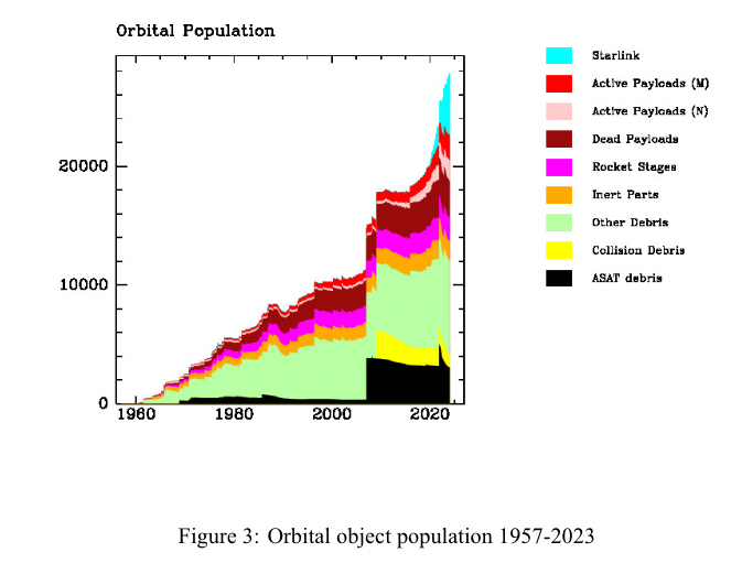
The figures below compare the two systems and show that the stereo technique acts to extend the distance between the telescope aperture and measurement plane, as though projecting the images to a negative altitude. The research led by Doris et al at the Advanced Instrumentation and Technology Centre at the Research School of Astronomy and Astrophysics (RSAA) at Mt Stromlo is novel in that it can capture high resolution data at high altitude, being able to measure effectively up to 20km into the atmosphere, using a single detector. 

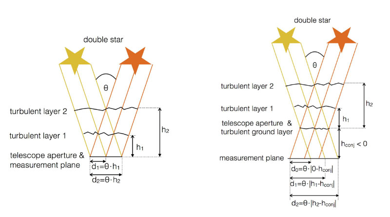
Above: Principle of conventional SCIDAR (left) – where the ground layer turbulence can’t be analysed, compared to generalised SCIDAR (right) – where the ground layer can be analysed due to the measurement plane at a negative altitude.

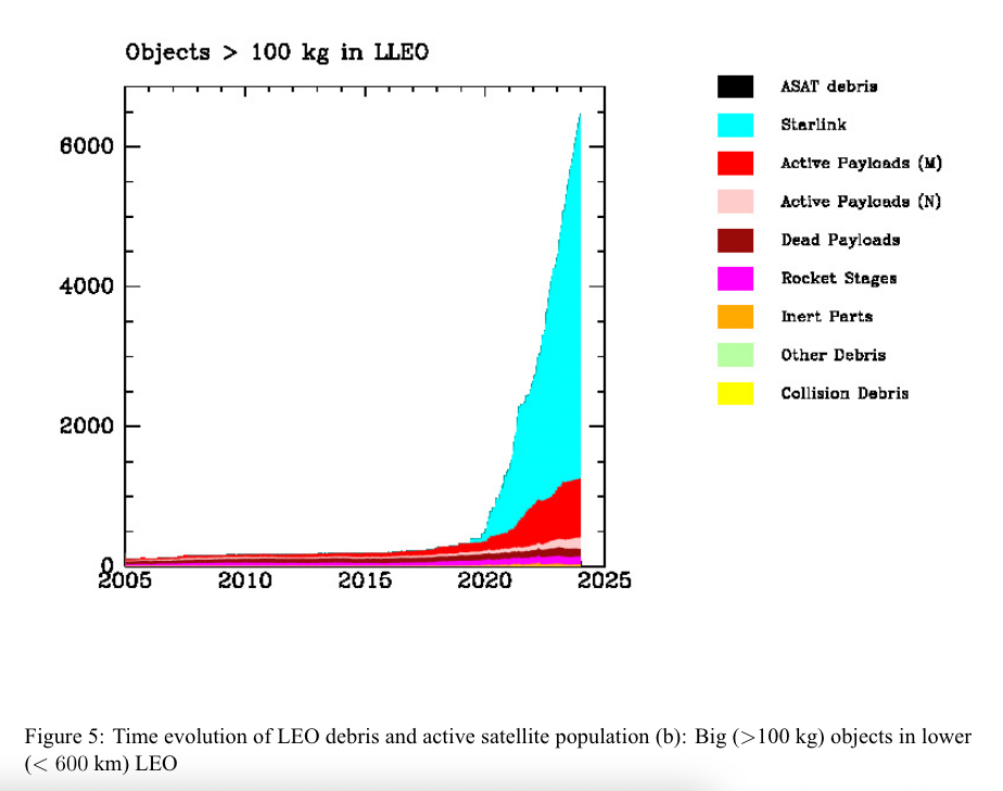
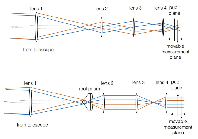
Schematic of the optical design of generalised SCIDAR (top) compared to stereo-SCIDAR with the addition of a roof prism (below).

Figures: Grosse, Doris, Francis Bennet, Visa Korkiakoski, Francois Rigaut, and Elliott Thorn. “Single Detector Stereo-SCIDAR for Mount Stromlo.” edited by Enrico Marchetti, Laird M. Close, and Jean-Pierre Véran, 99093D. Edinburgh, United Kingdom, 2016. https://doi.org/10.1117/12.2232149.

Night 1

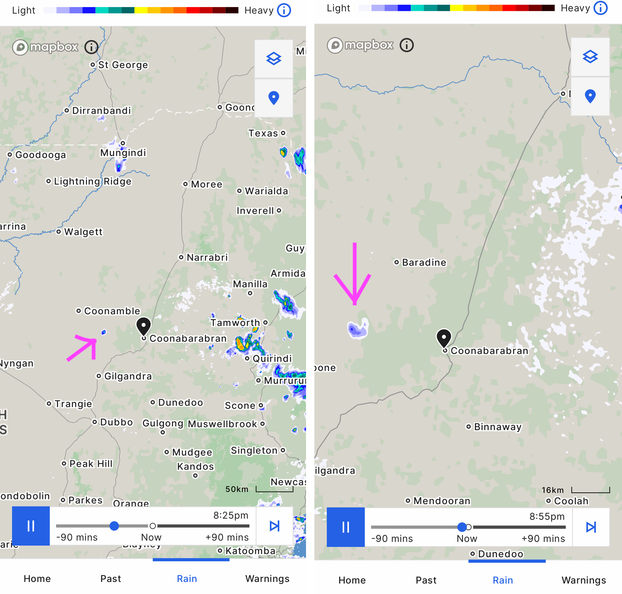
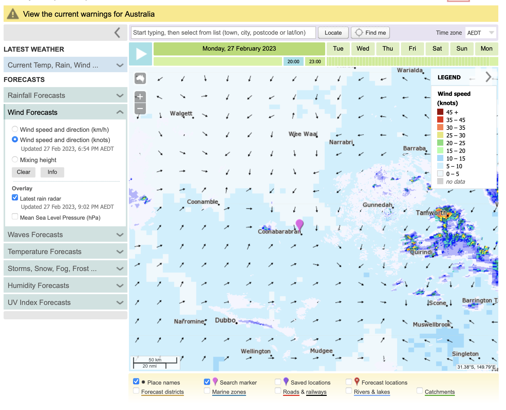
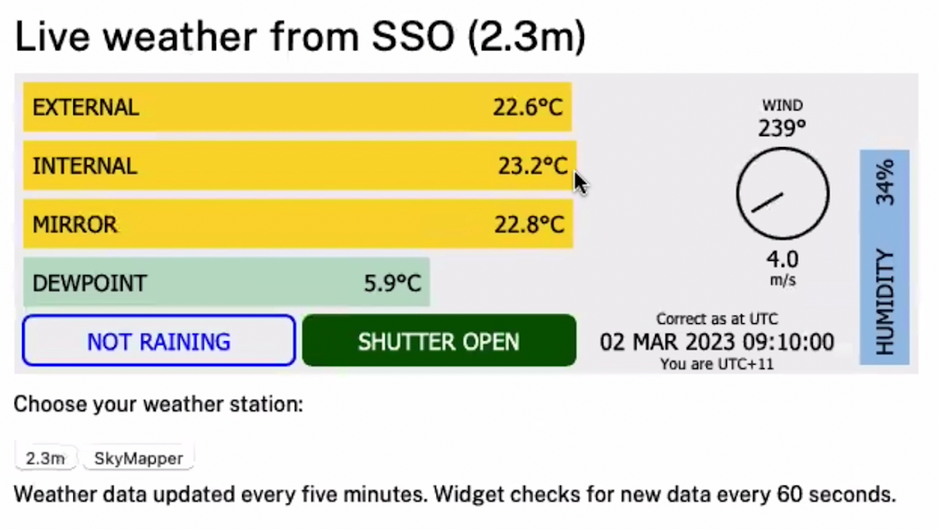
On the first night, we began by looking at the weather and rain radars for Siding Spring Observatory, Coonabarabran, in the Warrumbungles Dark Sky Park where the 2.3 metre telescope is located. This telescope is completely remotely operated (and about to become completely automated – not even operated by observers), and the entire building rotates as the telescope moves (!!).

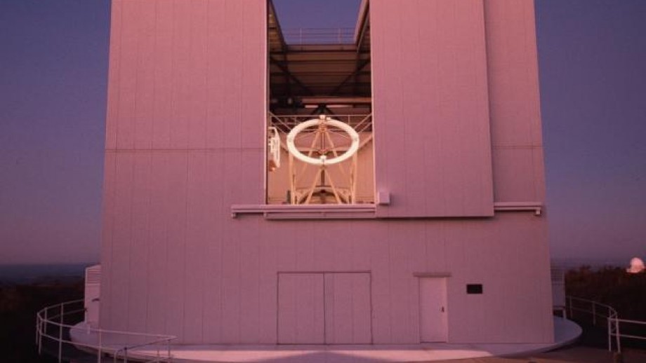
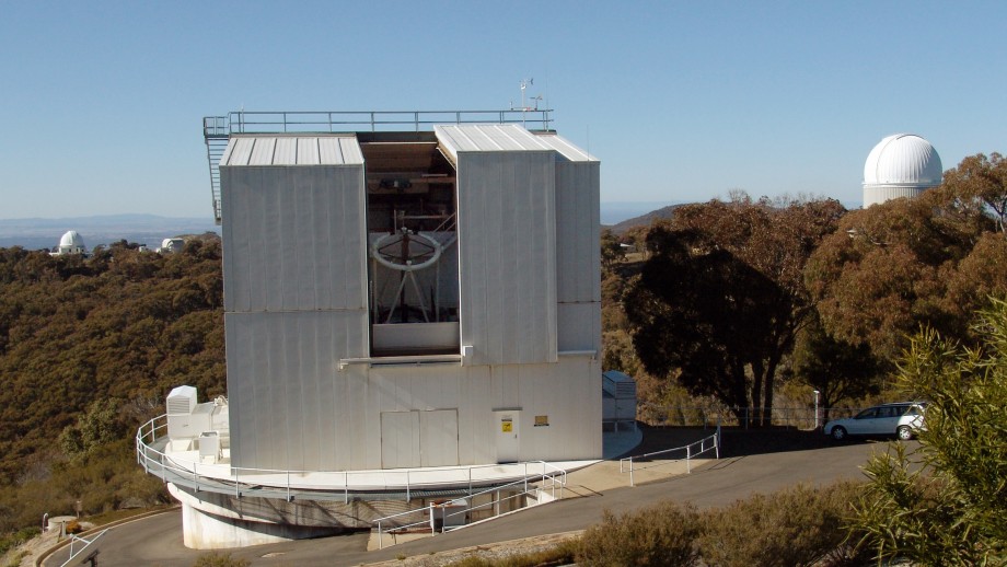
Images: https://rsaa.anu.edu.au/observatories/telescopes/anu-23m-telescope

The radar showed a few rain cells around the area, one in particular heading towards the telescope. Rain on the telescope can not happen, so observing is a no go if there is a chance of rain within 10km.

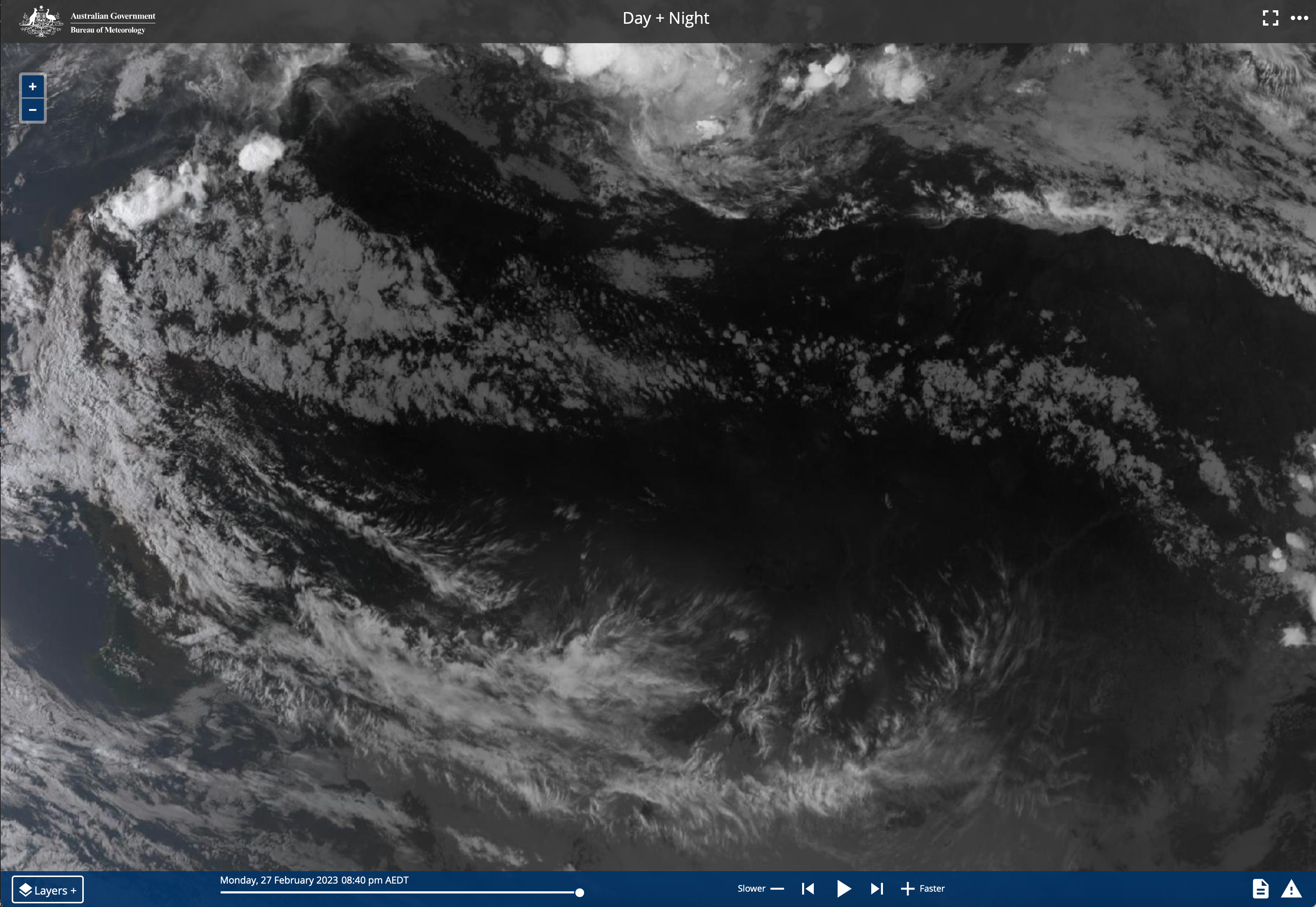
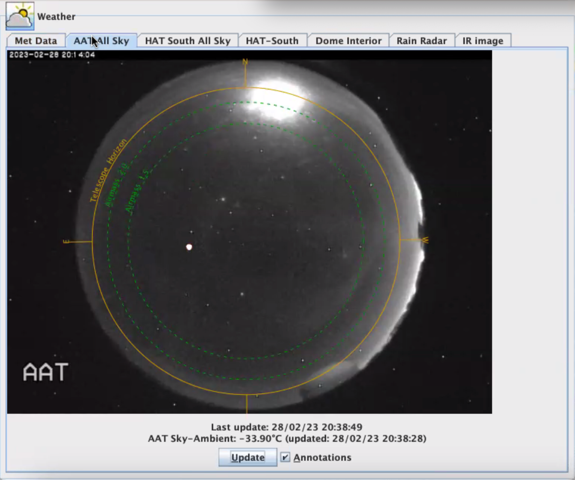
There are several places to get live meteorological data from SSO, as well as being able to check if the other telescopes on site were open and being used or not. Cross-checking this info with BOM rain radar, sat view, and wind sensors, Doris and Michael decided to hold off opening the telescope until later in the night. 


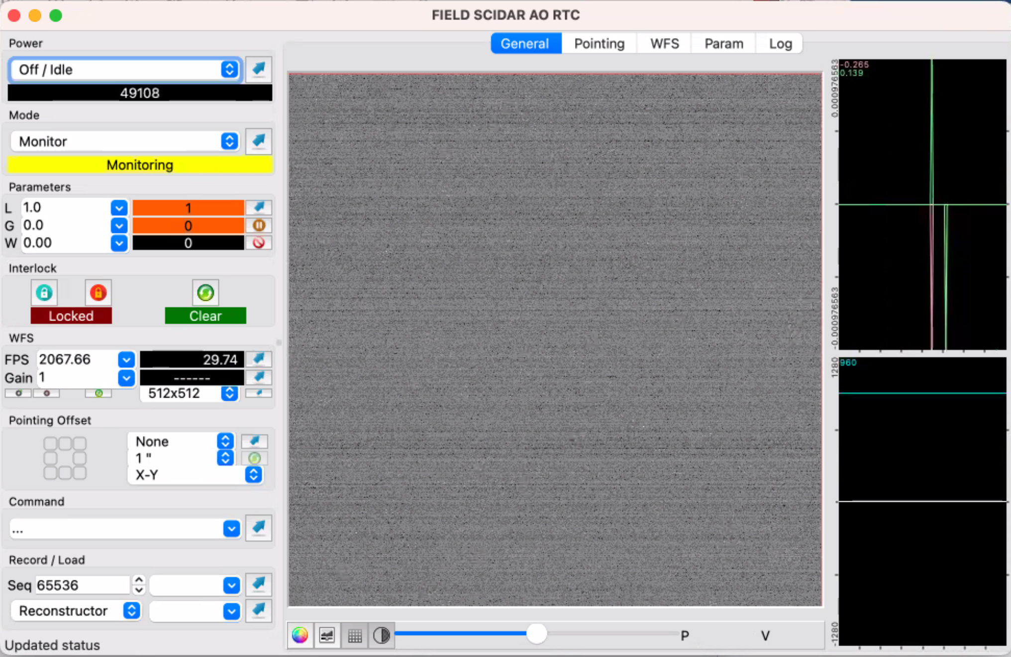
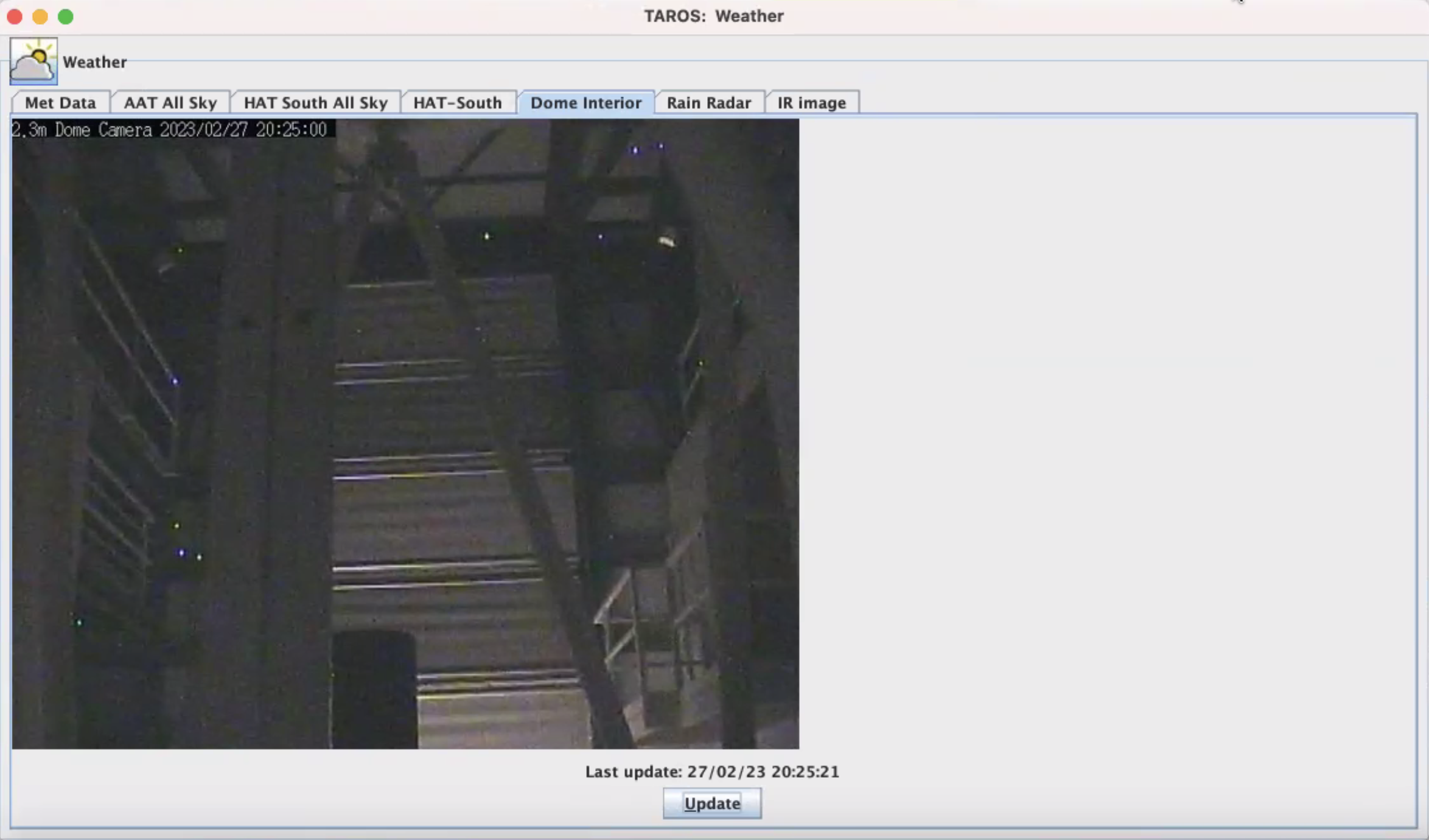
So the only view we got that night was of the inside of the telescope, but it was useful to get an introduction to the graphic user interfaces and to begin to understand the system – not just technically but also of humans and environmental factors that need to align to make this research happen.

Night 2

The second night was go! This was a clear night with no hesitation about the weather. After the software system is set up, the dome shutter is opened first.

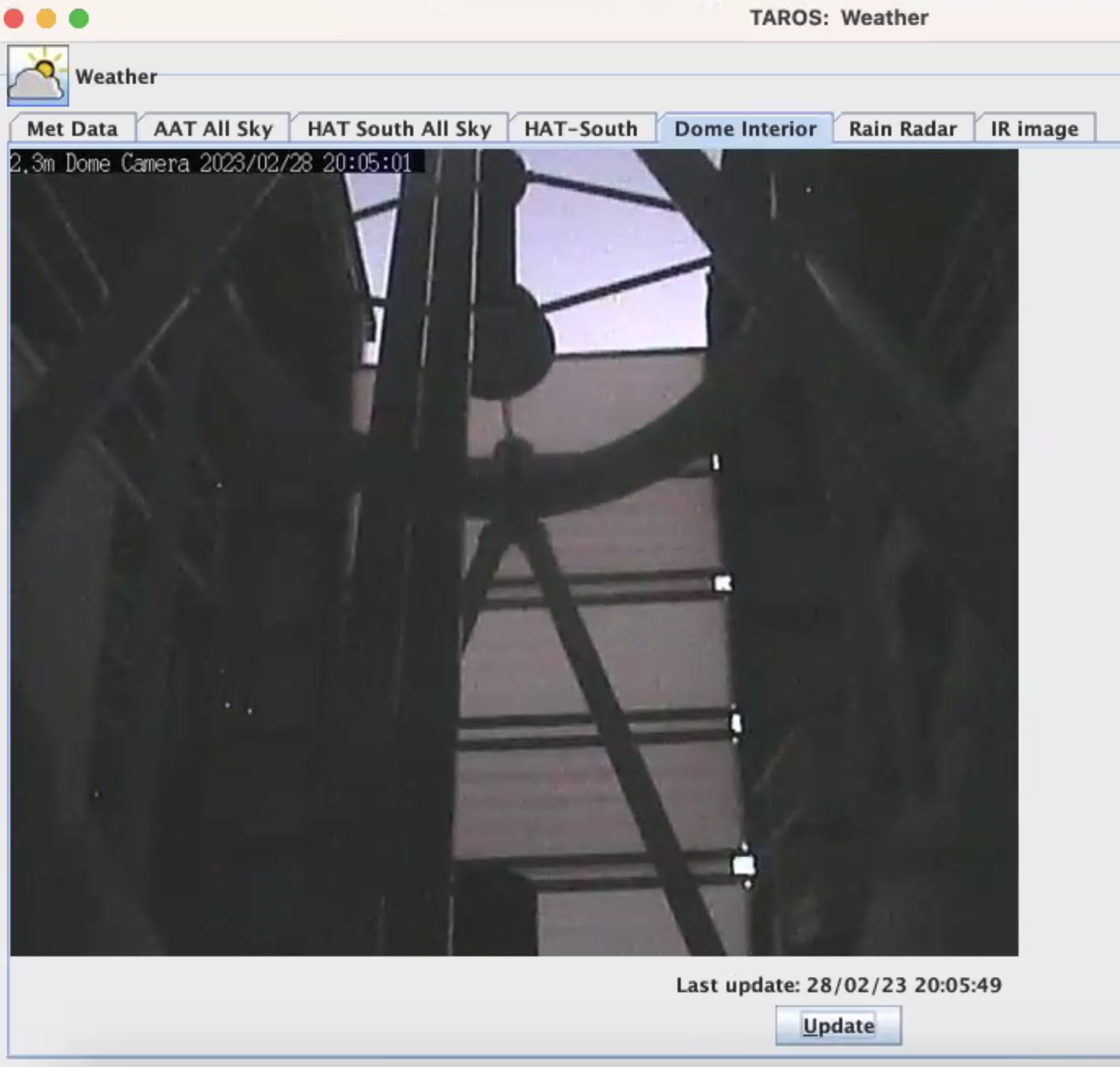
 After the dome shutter, the mirror covers can be opened, and this process can be seen on the screen with the sky and pupil image emerging as the telescope opens. 

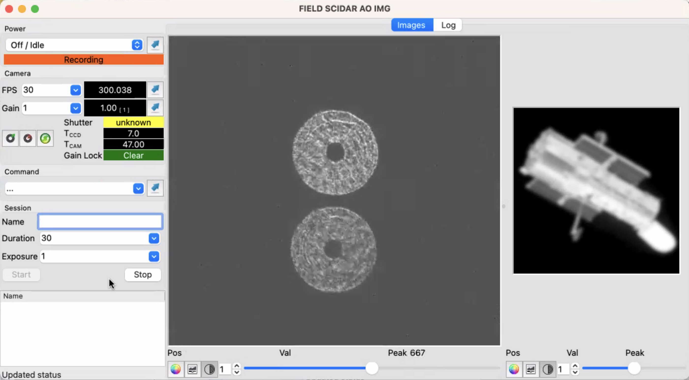
The pupil image is an image of the telescope’s aperture, which is obstructed by the mirror of the telescope held in place by ‘spider vanes’ which appear in clear images as cross hairs around the small circle in the centre.

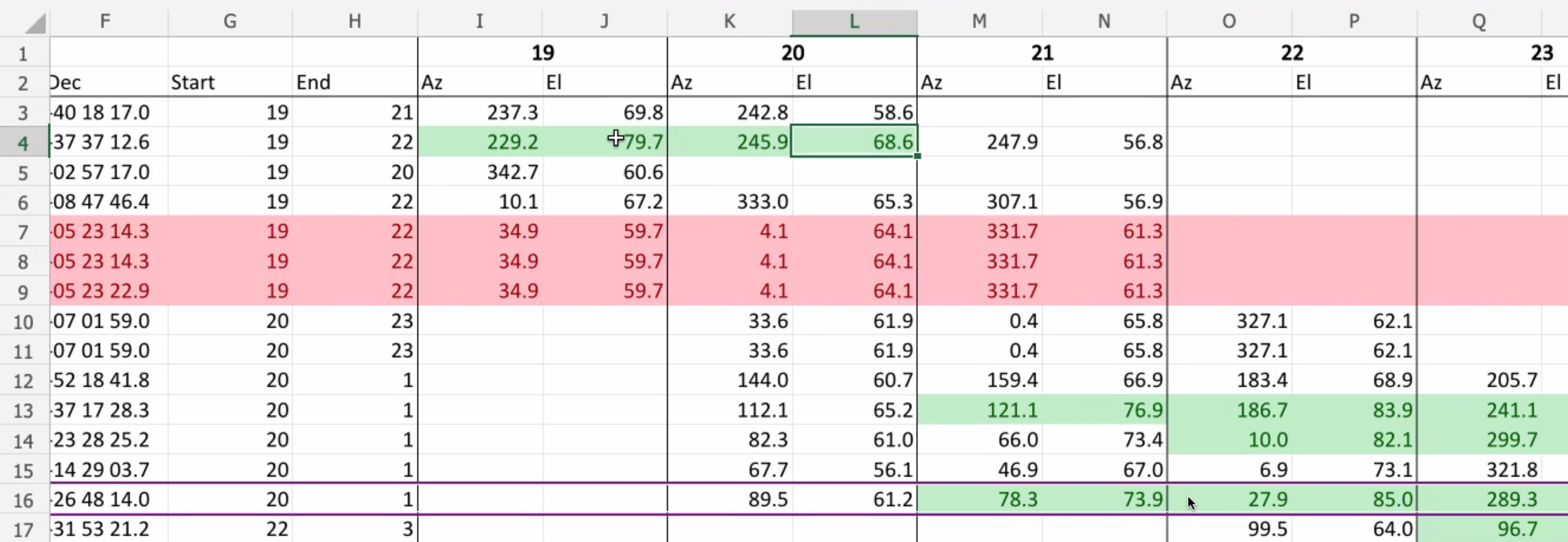
Michael and Doris had a list of double star coordinates to track. After tracking to the first double star, a different viewing window shows the acquisition image, which looks more like normal stars. At first, the stars were on an angle, so a position offset function was carried out to align them in a vertical orientation.


Positioning offset (sped up)

The stars are recorded in 10 minute intervals, to collect data that captures changes throughout the night. Over time, this data can compare turbulence throughout the year in response to seasonal change, as well as over El Niño and La Niña cycles.

After recording the first double star for 10 minutes, the telescope was set to move position onto the next set of coordinates. This takes up to a couple of minutes and after that amount of time we noticed it had stopped moving, and had encountered an error. 

Like all technological systems, there was a series of steps to try in a specific order, as well as the good old ‘turn off then on again’ trick. We spoke about other problems that have occurred, and the technical staff whose number you can call who can drive up and manually shut down the system. Luckily it didn’t come to that this time!

Night 3

The third night was clearer again, with the system set up and running quickly and smoothly.

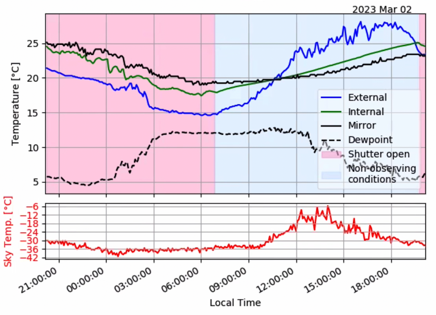
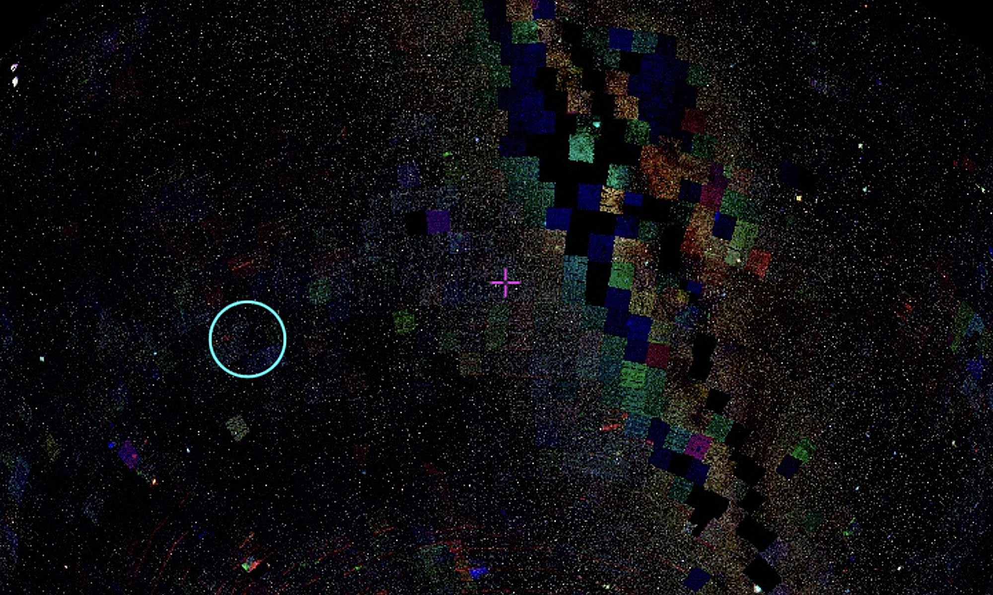
We went through the same process as the previous evening, and could see from the data various temperature changes and the use of the telescope for the previous 24 hours. The pink section indicates the telescope shutter was open and in use, signalling the previous nights work. We could also see the temperature difference between outside and inside the telescope, and at the mirror surface, was relatively low, which indicates good conditions.

This gave a nice clear view of both the pupil and acquisition images.

Tracking to a double star:

It was incredibly valuable to learn about this intricate and specialised research and experience the process of remote observing. It has given me new appreciation of the depth of knowledge involved at every step, and an insight into the characteristics and aesthetics of the network of humans and machines through which this practice operates.

A huge thank you Doris and Michael for sharing their time, process, and knowledge.

This research described in this blog post is supported by the Commonwealth of Australia as represented by the Defence Science and Technology Group of the Department of Defence.
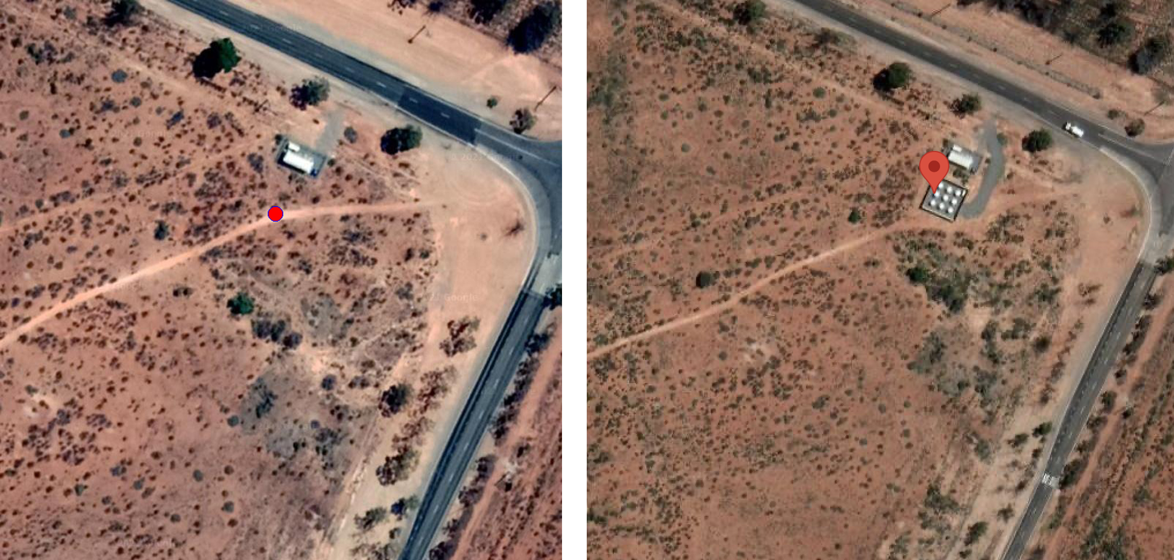
Signal to noise (mostly noise)

A big week of experimentation!

Using an antenna and RTL-SDR dongle, I have finally managed to receive data from weather satellites as they pass overhead and decode that signal into images. 

While still only a slice of image amongst a good amount of static, it was exciting to see some atmosphere emerge in these:

Process

RTL-SDR is a ‘software-defined’ radio scanner with a digital converter that allows access to the radio spectrum through a laptop.

Following Brad’s guidelines I was aiming to tune into the frequencies of National Oceanic and Atmospheric Administration (NOAA) satellites with CubicSDR, record the audio, then use WXtoImg to translate that audio file into a satellite image.

Software and set-up

The first hurdle was outdated and incompatible software. I ended up using noaa-apt image decoder instead of WXtoImg, installing it for MacOS using this tutorial and trying out Gqrx SDR for recording before going back to CubicSDR.

Frequencies

NOAA satellites are unlocked so anyone can access their data by tuning into the following signals:

    • NOAA 15: 137.62MHz
    • NOAA 18: 137.9125MHz
    • NOAA 19: 137.1MHz

Tracking satellite passes

To track these three NOAA satellites, I was using n2yo.com which shows the timing and maps of their predicted passes. I had to keep reminding myself that ‘visible passes’ refers to us seeing the satellite (or their reflected sunlight at dusk / night time) where as I was aiming for the opposite, and that the ‘invisible’ passes in daylight would be better for seeing from the satellite’s perspective.

In hindsight, I have realised that my failed attempts were probably just because the satellites were way too far away. The pass shown in the map above was not close enough to get a useful signal, the successful ones were slightly closer than this.

Noise > Signal

These were many failed attempts where I captured recordings that gave errors or were just not satellites. For example..

Single line:

Blips:

Triple j playing Gang of Youths Live at the Wireless (a nice surprise and a gig I was actually at! – but not a weather satellite)

Recording the singe line or blip frequencies were giving me wav files full of static: 

Recording the single line or blip frequencies were giving me wav files full of static that would be decoded into images equally full of static or with occasional blocks of contrast.

Leaving the recording on for 4 hours before going out hours created an image 11 metres long 😂


Noise < Signal

After more experiments with different settings, sample rates, and bandwidth I finally encountered a defined, strong signal of both NOAA 15 and 19, which looked like this:


And sounded like this:

Note antenna set up on balcony cabled through dog door (convenient!)

I made three recordings like this which produced the following images using noaa-apt with varying processing settings. 

NOAA 15 with synced frames, without map overlay:


NOAA 15 with synced frames, histogram settings to increase contrast, and map overlay:

NOAA 19, no extra settings:


NOAA 19 with histogram and false colour applied:

NOAA 19 with synced frames, histogram and false colour applied:


Technical notes

The NOAA User’s Guide for Building and Operating Environmental Satellite Receiving Stations was useful for understanding some of the technical elements of this process.

Two channels

Automatic Picture Transmissions (APT) is designed to broadcast direct satellite imagery to low-cost ground receiving equipment, by sending only two channels of high-resolution imagery, which explains the double imagery produced.

“The two images that appear in the APT are selected from ground control and, during daylight passes, usually consist of the visual channel and one of the infrared channels. At night, two infrared images are usually found in the APT. Therefore, the final product from APT consists of two images, side by side, representing the same view of the Earth in two different spectral bands.”

APT signal is continuously transmitted, creating an image strip that represents the time of transmission as the satellite passes overhead.

Telemetry

“IR Telemetry – At the end of the IR line is a zone dedicated to telemetry information. This data is coded as step-like changes in brightness, resulting in a strip down the right side of the IR image made up of gray scale step “wedges.” This information is used for calibrating temperature data in the image.

Visible Light Telemetry – The visible scan line ends with a telemetry window similar, but not identical, to the IR telemetry wedges.”

Bandwidth

I played around a lot with the bandwidth in different recordings, trying to make it wide enough to get the right signal / noise ratio, by placing the grey area just around the signal. The NOAA user’s guide indicates it should be around 40 KHz which ended up being right for my recordings.

Other settings are described in Image Data Acquisition for NOAA 18 and NOAA 19 Weather Satellites Using QFH Antenna and RTL-SDR by Wiryadinata et al, 2018.

Now I’ve got the basics working I am hoping to use this process to look at both frequency interference (starting to look more at the unwanted signals with more intention) and also to think more deeply around the recursive relationship between what satellites see, and what we see of them.


Maps, grids, and trading cells

This post follows on from my last one about Spectrum as a Natural Resource.

ACMA’s Register for Radiocommunications licences shows the use of different frequency bands across Australia. I’ve been gathering images that show some of the ways spectrum is used and shared.

These are of the main spectrum bands and the areas they are licensed to be used in:

In sequence:

Quiet Zones

There are many interesting aspects to these maps, one of which is the gaps in spectrum use around radio quiet zones for astronomy research. The Radiocommunications Assignment and Licensing Instructions (RALI) is designed for services that operate within the frequency bands:

    • 1250 – 1780 MHz
    • 2200 – 2550 MHz
    • 4350 – 6700 MHz
    • 8000 – 9200 MHz
    • 16 – 26 GHz

The prescribed zones of CSIRO facilities are at:

    • Parkes (NSW)
    • Narrabri (NSW)
    • Coonabarabran (NSW)
    • Hobart (Tas)
    • Ceduna (SA)
    • Tidbinbilla (ACT)

This is Tidbinbilla quiet zone:

And the SKA site in WA:

Viasat and Starlink

I noticed one layer of the maps above that was different to any other, and found that this license is owned by Viasat. It is an Area Wide License (AWL) for fixed satellite services, introduced in 2020.

A sample of the list of licenses held by SpaceX in ACMA’s register:

Starlink licences can be seen on the map for the ground station sites I wrote about in a previous post. 

A viewshed “shows line-of-sight visibility between a transmitter and multiple receivers in a given radius and direction.” It is therefore used to determine signal reach and interference.

This is the 30km viewshed for the Starlink ground stations at BullaBulling, WA:

The Grid

Spectrum is divided into a grid system for allocation that uses a ‘hierarchical cell identification scheme’ (HCIS) to define different geographic areas.

The grid is divided into 5 x 5-minute of arc cells (approx. 9km square) Australia-wide. This was updated in 2020 to “allow far greater granularity in the description of areas and, in many cases, the ability to trade smaller areas, particularly in regional Australia.”

Spectrum licences are for geographic areas that are defined by these cells. For areas that need to be broken down into smaller areas, the grid can be subdivided into ‘extensions’, where the cells are first divided into 25 cells of 1 × 1 minutes of arc (approx 1.8 km square), then 12 cells each 20 × 15 seconds of arc (approx 500m square).

Presumably this is what is happening around high-density areas where the spectrum is divided differently around highly-populated areas for greater need of certain frequencies.

Auctions

As I wrote about earlier, Australia uses an auctioning systems to allocate spectrum depending on the specific spectrum characteristics, use, and demand. The results are published on the ACMA website, for example these are the auction results for the 850/900 MHz and 26GHz bands in 2021:

Trading

Spectrum licences for single HCIS cells can be traded as ‘Spectrum trading units’. The standard bandwidth of one STU is 1Hz but it can be combined with another STU vertically to increase bandwidth or horizontal to cover a larger area. 

Tectonic plates!    

I was fascinated to find that the datum system (a mathematical coordinate system that takes into account the uneven shape of the earth) for the spectrum grid needs to be updated because of tectonic plate movement:

“The need to update arises from the motion of the Australian tectonic plate in a roughly north-north-east direction at approximately 7 cm per year. The coordinate discrepancy between GDA94 and GDA2020 varies from approximately 1.5 m in south-eastern Australia, to approximately 1.8 m in north-western Australia.”

This seems a fitting reminer that our technical systems and standards are built on natural foundations that we need to recalibrate to across time and space.

I could go on relaying random facts like this, but instead I am going to use an antenna that Brad gave me to tune into and hopefully download images from weather satellites as they pass overhead.  More on that soon!

Spectrum as a Natural Resource

I’ve taken a bit of a detour this week to explore broader discourse around the electromagnetic spectrum. Obviously this is a HUGE topic so I am only scratching the surface but there are a few things I have found fascinating.

I am interested in how the electromagnetic spectrum is classified as a limited natural resource. This seems at odds with how it is perceived as ubiquitous – or not even considered – in contemporary culture that is built on technologies that rely on it. Similarly, the communication and connectivity that spectrum provides is intrinsically linked to cultural and social values, but it is more commonly treated as an economic and technological commodity.

Sharing spectrum

The full electromagnetic spectrum ranges from gamma rays to radio waves, and the part of that range with frequency range from 30 Hz to 300 GHz makes up the radio spectrum. Different parts of the spectrum have different qualities so are allocated to different uses.

Basic examples are:

    • Higher frequencies are shorter radio waves that carry more information.
    • Lower frequencies are longer waves that carry less information.
    • Lower frequencies travel close to the ground and are generally used by the military. 
    • Higher frequencies travel at greater heights reaching orbiting satellites.

Because of the different characteristics of different frequencies, there are a range of factors involved in how the spectrum is used, shared, exploited, and constrained over time and space.

“The same frequency can be used in different geographical areas, depending on its propagation characteristics; or the same frequency can be used in the same area, but at different times. Or two different frequencies can be used in the same area at the same time…. the cardinal constraint on the use of the radio spectrum is interference-interference with someone else’s use by communicating on the same frequency at the same time and the same place.” (Herter, p. 655)

Renewable and pollutable

Similarities and differences are drawn between spectrum and other natural resources like water, trees, minerals, and air.  As such, “ecological equilibria exist for this resource just as they do elsewhere in nature” (Ryan). 

A significant difference between spectrum and other natural resources is that it is instantly renewable.

“Unlike hard minerals or petroleum, the electromagnetic spectrum is not depletable; it is always available in infinite abundance except for that portion which is being used. When that portion of the electromagnetic spectrum is not in use, it is instantly renewable.” (Herter, p. 653)

However, a strong similarity is that it can be polluted, wasted, or abused, and it is frequently subject to overcrowding causing interference that prevents it being used effectively.

“The spectrum has been called a “limited” natural resource because, given present technology, there is only a finite portion available for beneficial uses at any one time.” (Herter, p. 655)

Another element at play is that as demand for radio spectrum increases, technologies are developed to use it more efficiently by operating at higher bandwidths.

Global Commons

Gregory and Taylor’s research brings together a range of perspectives on the “constantly morphing policy puzzle” of radio spectrum from around the world to create an interdisciplinary dialogue around radio spectrum:

“Spectrum policy is a field on which academics – especially in the social sciences and humanities – often fear to tread. But why? The current policy climate surrounding spectrum policy will clearly benefit from what the arts and humanities have to offer.” (Taylor and Middleton, p. 8)

They challenge the power dynamics in current approaches to access and affordability of mobile communication with a reminder that spectrum is a public resource. However, “Instead of recognizing this resource as such, the United States and countries in Europe relegate the management and supervision of this natural resource to technocrats who deal with telecommunications.” (Ryan)

In New Zealand, an agreement has been reached for management of the spectrum to be shared between government and Māori partners after a decades-long debate over spectrum rights.

Māori groups consider spectrum a cultural more than technological phenomenon: one that is intrinsic in supporting language and culture just as much as economic development. It is therefore regarded as ‘a taonga, a treasure’” (Joyce, p. 25)

Zita Joyce writes: “the story of New Zealand radio spectrum is about the limits of the property rights regime. More fundamentally, it is about the right of the state to create property rights in previously unpropertized resources, and the right of Indigenous peoples to challenge this propertization, posing traditional forms of knowledge and resource use against state discourses of technology and material value.” (Joyce, p. 38)

Australian spectrum allocation

Spectrum in Australia is managed by the Australian Communication and Media Authority (ACMA) and primarily licensed through auctions. 

Their Register of Radiocommunications Licences shows who uses which frequencies where, which is what led me into this rabbit hole in the first place, so I am going to write about this in a separate post!

References

Joyce, Zita. “Radio spectrum as Indigenous space: Property rights and traditional knowledge in New Zealand’s spectrum.” Frequencies: International spectrum policy (2020): 19-45.

Herter Jr, Christian A. “The electromagnetic spectrum: A critical natural resource.” Nat. Resources J. 25 (1985): 651.

Ryan, Patrick S. “Treating the wireless spectrum as a natural resource.” Envtl. L. Rep. News & Analysis 35 (2005): 10620.

Taylor, Gregory, and Catherine Middleton, eds. Frequencies: International Spectrum Policy. McGill-Queen’s Press-MQUP, 2020.

Groundstations

While trawling https://satellitemap.space/, I came across details about and images of Starlink groundstations. Groundstations, or gateways, connect Starlink satellites to existing fibre-optic infrastructure. Borrowing this succinct explanation:

So, a user’s home antenna connects to a Starlink satellite as it passes overhead, which in turn links them into the nearest gateway. As a result, in addition to their own antenna, users need to have a ground station within roughly 500 miles of their location to get service.” 

This database includes the GPS locations, number of antennas and their diameters, manufacturer, and uplink and downlink frequencies, as well as a satellite photo of their location.

Data about the Starlink grounstation in Cobargo, NSW

Interestingly, most (but not all) of these satellite images were taken before the ground stations were built. Searching the lat/long coordinates on Google Earth often gave a more recent satellite view, showing the ground station appearing in the landscape.

In a similar way to how the same star is recorded at different times to observe change in astronomy, satellite imagery captures the emergence of these antennas on the land.

Broken Hill, NSW.


Ki Ki, South Australia


TeHana, New Zealand


Warren, Missouri, US

These images show the physical presence of megaconstellations in our natural and built environment, and renewed my interest in how this may impact the land and ecosystem.

This Google map plots ground stations and the areas they cover. All US gateways filed with the FCC are on the map. In other countries most likely not all gateways are shown.

In similar combinations of sources that I have been using, it uses the imagery of satellites to visualise their own proliferation.

An extra link on each of these groundstation database pages referred me to the relevant radiocommunications licence – in Australia, this is administered by the Australian Communications and Media Authority (ACMA). This led me into a huge rabbit hole of reading about radio frequency allocation, which will be my next post!

Orbits

Following the previous video combining natural and artificial constellations, I keep searching for a way to visualise the paradox of images and data that satellites both generate, and contaminate.

I asked Brad if there was a way to see a live view of the satellites passing an exact location using RA / dec coordinates. While not exactly what I’m looking for, this site generates live sky views that includes both natural and artificial sky objects. It also shows the orbits of satellites as you select them. 

I wanted to expand on my previous video to also include the ‘inverted astronomy’ that Gärdebo et al and Sloterdjik describe as ‘looking down from space onto the earth rather than from the ground up into the skies’, to synthesise images that satellites provide, with the presence of them as we look to the skies. 

This animation combines a satellite image of the location that I generated the sky view for, combined with satellite and star positions at the time I took this screen recording.

Compared to my last video, this one includes the ‘looking down’ perspective in terms of imagery, but leaves out the visualisation of the internet coverage the satellites provide. Also, drawing in the satellites’ orbital lines indicates the streaks they leave on astronomical images.

Starlink orbital shells

Anthony Mallama’s research shows how Starlink satellites will create eight orbital ‘shells’ at different altitudes. Examples of these shells at medium and high inclination are shown here: 

Diagrams of the orbital shells of Starlink megaconstellations

Orbital Debris Reentry Predictions

Orbits are also interesting because their exact path over time is unstable due to atmospheric drag, solar wind, and gravitational pull, which is why space debris is hitting the earth at unpredictable locations.

Re-entry prediction map

Image: Reentry prediction from the Aerospace Center for Orbital and Reentry Debris Studies on 3 Nov for the Long March 5B rocket body launched 31 Oct. Credit: The Aerospace Corporation